Introduction to Fourier transform
The definition of Fourier transform (FT) is the given by
Normally, f(r) is real for all $\mathrm{\textbf{r}}\in\mathrm{\textbf{R}}$, and its Fourier tranform F(k) is complex, having both the real and imaginary parts. Typically, only the modulus of F(k) is analyzed, and the phase (complex angle) of F(k) is discarded.
In general, the information in f(r) can be fully recovered from F(k). More explicitly,
in the intensity map (the modulus of F(k)): intensity –> amplitude of features/oscillations k vector –> oscillation wavevector profile –> type of features/oscillations (e.g. sine wave vs square wave) in the phase map: Phase (angle of complex number) –> locations of features/oscillations in f(r) and types of features/oscillations (e.g. sine vs cosine wave with the same amplitude and frequency) In this brief summary, I would like to particularly focus on the relation between the phases of FT and the locations of features/oscillations in r-space.
An example showing the importance of phase
(Part of this section refers to the very informative introduction by Randy J. Read http://www-structmed.cimr.cam.ac.uk/Course/Fourier/Fourier.html.)
The following code shows that important information can be stored in the phases, following Fourier transformation. At the top of Figure 1, the photographs of Albert Einstein (left) and a raccoon (right) are shown. We can treat the photographs as density maps and calculate their FTs, to obtain intensities (amplitudes) and phases.
import numpy as np
from scipy import misc
from scipy import interpolate
import matplotlib.pyplot as plt

# read the image of Einstein, image source: http://cdn.nrm.com.mx/cdn/secreto/2016/imagenes/contenido/albert.jpg
Einstein = misc.imread("Albert_Einstein_Head.jpg")
Einstein2 = Einstein[:,:,0]  # get only one layer of RGB photograph which is gray anyway
Einsteinfft = np.fft.fft2(Einstein2)  # FT the photograph
# read the image of a racoon, from scipy's package
face = misc.face(gray=True).astype(float)
face2 = face[0:500, 350:850]  # get a 500X500 pixels image, same to the size of Einstein's image
face2fft = np.fft.fft2(face2)  # FT

# exchange the phase maps, and inverse FT
face2fftinv = np.fft.ifft2(np.multiply(abs(face2fft),np.exp(1j*np.angle(Einsteinfft))))#Einsteinfft)))
Einsteinfftinv = np.fft.ifft2(np.multiply(abs(Einsteinfft),np.exp(1j*np.angle(face2fft))))

# plot data
fig, ((ax1, ax2), (ax3, ax4)) = plt.subplots(2, 2, sharex='col', sharey='row',figsize = (12, 10))
ax1.imshow(Einstein2, cmap=plt.cm.gray)
ax1.set_title("Einstein")
ax1.axis("off")
ax2.imshow(face2,cmap=plt.cm.gray)
ax2.set_title("Raccoon")
ax2.axis("off")
ax3.imshow(np.abs(Einsteinfftinv), cmap=plt.cm.gray)
ax3.set_title("Einstein Intensity with Raccoon Phase")
ax3.axis("off")
ax4.imshow(np.abs(face2fftinv), cmap=plt.cm.gray)
ax4.set_title("Racoon Intensity with Einstein Phase")
ax4.axis("off")
fig.suptitle("Figure 1", fontsize=14, fontweight='bold')

plt.show()
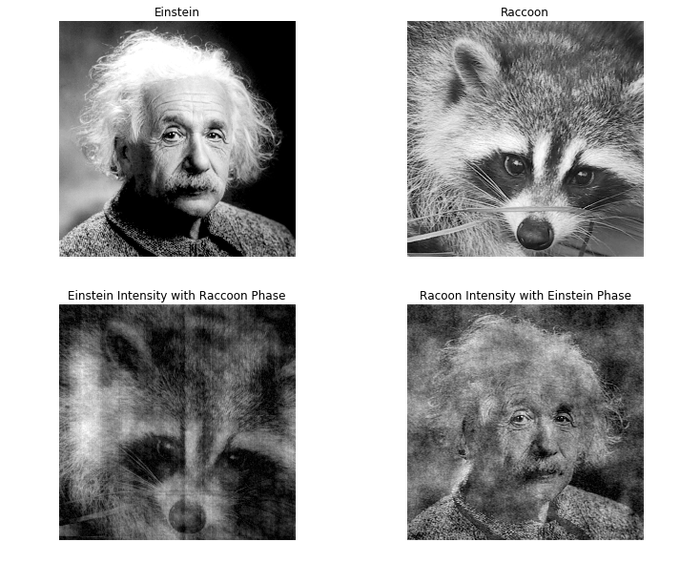
If the phases of the FT were exchanged, namely inverse Fourier transforming the Einstein intensity map with the raccoon’s phases and vice versa, we obtain the pictures at the bottom of Figure 1. Dramatically, one can clearly identify a raccoon from the left graph (the inverse FT of the Einstein intensity map with the raccoon’s phases) and Einstein from the right graph (the inverse FT of the raccoon’s intensity map with the Einstein’s phases). The phases dominate what we see in r-space.
The phase of FT and Locations of Features/Oscillations To understand the origin of this effect, we Fourier transfrom a simple 1D wave-packet at different locations, as shown in the following code and figure.
%matplotlib inline

# Define Gaussian function to be used profiling a gaussian wave-packet.
def gauss(x, A = 1, mu = 0, sigma = 1):
    return A*np.exp(-(x-mu)**2/(2.*sigma**2))

# Plot function
def plotFT(x, k, testData, testDataFFT, ax1, ax2, ax3, addTitle = False):
    ax1.plot(x, testData)
    ax1.set_xlabel('x')
    ax1.set_ylabel('amplitude')
    if addTitle == True:
    ax1.set_title('Oscillations')
    ax1.set_xlim([0, 100])

    ax2.plot(k, np.fft.fftshift( np.abs(testDataFFT)))
    ax2.set_xlabel('k')
    ax2.set_ylabel('Intensity')
    if addTitle == True:
    ax2.set_title('Intensity of Fourier Transform')
    ax2.set_xlim([-2, 2])

    ax3.plot(k, np.fft.fftshift( np.angle(testDataFFT)))
    ax3.set_xlabel('k')
    ax3.set_ylabel('phase')
    if addTitle == True:
    ax3.set_title('Phase of Fourier Transform')
    ax3.set_xlim([-2, 2])


# forming a wave-packet and FT
x = np.arange(0,100,0.5)
k = np.arange(-2*np.pi, 2*np.pi, 0.02*np.pi)
testData1 = np.multiply(np.cos(x),gauss(x, mu = 30, sigma = 10))
testData1FFT = np.fft.fft(testData1)
# move the wave-packet to the second location
testData2 = np.multiply(np.cos(x-20),gauss(x, mu = 50, sigma = 10))
testData2FFT = np.fft.fft(testData2)
# move the wave-packet to the third location
testData3 = np.multiply(np.cos(x-40),gauss(x, mu = 70, sigma = 10))
testData3FFT = np.fft.fft(testData3)

# show the results
fig, ((ax1, ax2, ax3),(ax4, ax5, ax6),(ax7, ax8,
    ax9)) = plt.subplots(3, 3, figsize = (12, 12))
plotFT(x, k, testData1, testData1FFT,ax1, ax2, ax3,addTitle = True)
plotFT(x, k, testData2, testData2FFT,ax4, ax5, ax6)
plotFT(x, k, testData3, testData3FFT,ax7, ax8, ax9)
fig.suptitle("Figure 2", fontsize=14, fontweight='bold')

plt.show()
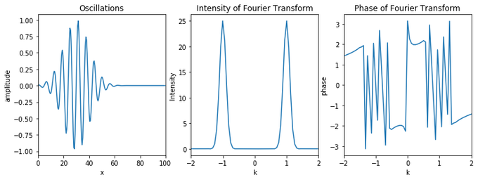
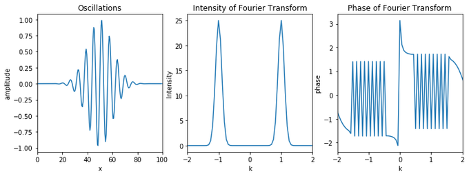
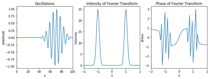
We can see that, for the same wave-packet, different locations yield very different phases while the intensity curve remains unchanged. Therefore, for the same feature/oscillation, the location information in r-space is primarily stored in k-space phases.
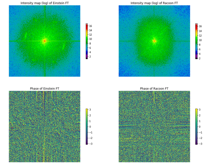
Let us come back to the photographs and compare the FT of the two images, as shown in the following code and figure. The photographs consist of spikes and terraces whose FT intensity maps are broadened domes centered at k = (0,0) (see the Figure 3). However, the phase maps, storing the locations of these spikes and terraces, look quite different in their fine structures. Therefore, by exchanging the phases of the two FT with similar intensity maps, the image in the inverse FT is dominated by the phases.
In summary, if only the frequency/wavevector, amplitudes, and types of features are concerned, analyzing the intensity map should be enough most of the time. However, if one wants the locations of the features/oscillations, the phase map should not be ignored.
# plot the intensity maps and phase maps of FT of Einstein's image and the racoon's image
fig, ((ax1, ax2), (ax3, ax4)) = plt.subplots(2, 2, sharex='col', sharey='row',figsize = (15, 12))
fig.suptitle("Figure 3", fontsize=14, fontweight='bold')
graph1 = ax1.imshow(np.fft.fftshift(np.log(np.abs(Einsteinfft))), cmap=plt.cm.spectral)
ax1.set_title("Intensity map (log) of Einstein FT")
ax1.axis("off")
fig.colorbar(graph1, ax=ax1, shrink=0.5)
ax1.set_aspect('equal')

graph2 = ax2.imshow(np.fft.fftshift(np.log(abs(face2fft))),cmap=plt.cm.spectral)
ax2.set_title("Intensity map (log) of Racoon FT")
ax2.axis("off")
fig.colorbar(graph2, ax=ax2, shrink=0.5)
ax2.set_aspect('equal')

graph3 = ax3.imshow(np.fft.fftshift(np.angle(Einsteinfft)), cmap=plt.cm.viridis)
ax3.set_title("Phase of Einstein FT")
ax3.axis("off")
fig.colorbar(graph3, ax=ax3, shrink=0.5)
ax3.set_aspect('equal')

graph4 = ax4.imshow(np.fft.fftshift(np.angle(face2fft)), cmap=plt.cm.viridis)
ax4.set_title("Phase of Racoon FT")
ax4.axis("off")
fig.colorbar(graph4, ax=ax4, shrink=0.5)
ax4.set_aspect('equal')

plt.show()